Brexit Data Project

Challenge 1: Brexit plot
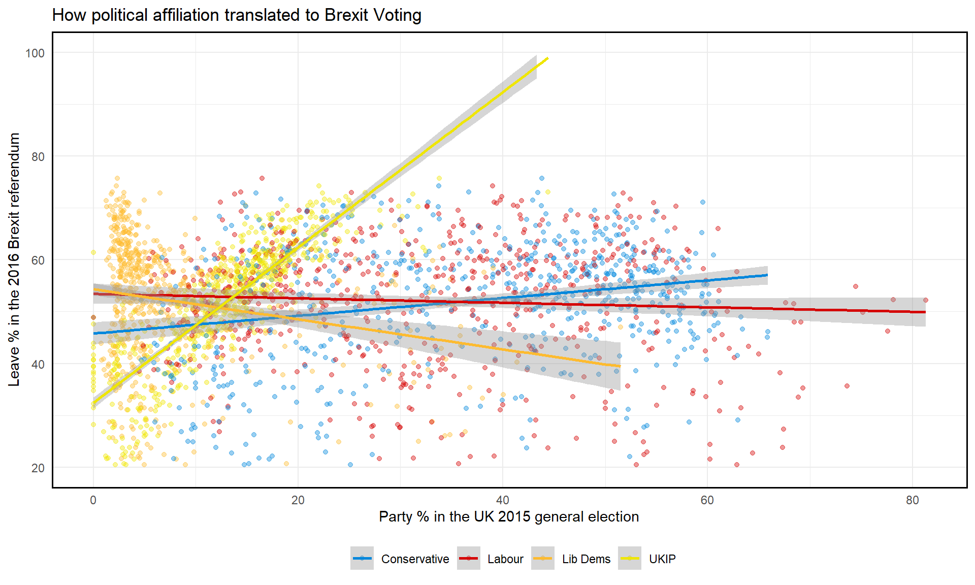
The graph shows how party affiliation affected votes for Brexit. It is evident that UK Independence party supporters had the highest votes for Brexit. The analysis of data shows the predictability of a brexit like vote based on political affiliations and this could lead to parties making laws based on predictive affiliations rather than pure good of the nation.
# Load data
brexit <- read_csv(here::here("data", "brexit_results.csv"))

# Inspect data
glimpse(brexit)
## Rows: 632
## Columns: 11
## $ Seat <chr> "Aldershot", "Aldridge-Brownhills", "Altrincham and Sale W~
## $ con_2015 <dbl> 50.6, 52.0, 53.0, 44.0, 60.8, 22.4, 52.5, 22.1, 50.7, 53.0~
## $ lab_2015 <dbl> 18.3, 22.4, 26.7, 34.8, 11.2, 41.0, 18.4, 49.8, 15.1, 21.3~
## $ ld_2015 <dbl> 8.82, 3.37, 8.38, 2.98, 7.19, 14.83, 5.98, 2.42, 10.62, 5.~
## $ ukip_2015 <dbl> 17.87, 19.62, 8.01, 15.89, 14.44, 21.41, 18.82, 21.76, 19.~
## $ leave_share <dbl> 57.9, 67.8, 38.6, 65.3, 49.7, 70.5, 59.9, 61.8, 51.8, 50.3~
## $ born_in_uk <dbl> 83.1, 96.1, 90.5, 97.3, 93.3, 97.0, 90.5, 90.7, 87.0, 88.8~
## $ male <dbl> 49.9, 48.9, 48.9, 49.2, 48.0, 49.2, 48.5, 49.2, 49.5, 49.5~
## $ unemployed <dbl> 3.64, 4.55, 3.04, 4.26, 2.47, 4.74, 3.69, 5.11, 3.39, 2.93~
## $ degree <dbl> 13.87, 9.97, 28.60, 9.34, 18.78, 6.09, 13.12, 7.90, 17.80,~
## $ age_18to24 <dbl> 9.41, 7.33, 6.44, 7.75, 5.73, 8.21, 7.82, 8.94, 7.56, 7.61~skim(brexit)| Name | brexit |
| Number of rows | 632 |
| Number of columns | 11 |
| _______________________ | |
| Column type frequency: | |
| character | 1 |
| numeric | 10 |
| ________________________ | |
| Group variables | None |
Variable type: character
| skim_variable | n_missing | complete_rate | min | max | empty | n_unique | whitespace |
|---|---|---|---|---|---|---|---|
| Seat | 0 | 1 | 4 | 43 | 0 | 632 | 0 |
Variable type: numeric
| skim_variable | n_missing | complete_rate | mean | sd | p0 | p25 | p50 | p75 | p100 | hist |
|---|---|---|---|---|---|---|---|---|---|---|
| con_2015 | 0 | 1.00 | 36.60 | 16.22 | 0.00 | 22.09 | 40.85 | 50.84 | 65.88 | ▂▅▃▇▅ |
| lab_2015 | 0 | 1.00 | 32.30 | 16.54 | 0.00 | 17.67 | 31.20 | 44.37 | 81.30 | ▆▇▇▅▁ |
| ld_2015 | 0 | 1.00 | 7.81 | 8.36 | 0.00 | 2.97 | 4.58 | 8.57 | 51.49 | ▇▁▁▁▁ |
| ukip_2015 | 0 | 1.00 | 13.10 | 6.47 | 0.00 | 9.19 | 13.73 | 17.11 | 44.43 | ▃▇▃▁▁ |
| leave_share | 0 | 1.00 | 52.06 | 11.44 | 20.48 | 45.33 | 53.69 | 60.15 | 75.65 | ▂▂▆▇▂ |
| born_in_uk | 0 | 1.00 | 88.15 | 11.29 | 40.73 | 86.42 | 92.48 | 95.42 | 98.02 | ▁▁▁▂▇ |
| male | 0 | 1.00 | 49.07 | 0.80 | 46.86 | 48.61 | 49.02 | 49.43 | 53.05 | ▁▇▃▁▁ |
| unemployed | 0 | 1.00 | 4.37 | 1.42 | 1.84 | 3.23 | 4.19 | 5.21 | 9.53 | ▆▇▅▂▁ |
| degree | 59 | 0.91 | 16.71 | 8.36 | 5.10 | 10.79 | 14.69 | 19.59 | 51.10 | ▇▆▂▁▁ |
| age_18to24 | 0 | 1.00 | 9.29 | 3.59 | 5.73 | 7.30 | 8.28 | 9.60 | 32.68 | ▇▁▁▁▁ |
# Change to long format
brexit_long <- brexit %>%
  pivot_longer(cols=c('con_2015', 'lab_2015', 'ld_2015', 'ukip_2015'), names_to= "Party",
               values_to="Party_share")

# Plot graphs group/colour based on party
ggplot(data=brexit_long, aes(x=Party_share, y=leave_share, group=Party, colour=Party)) +

  # Set colour
  scale_color_manual(values = c("#0087dc", "#d50000", "#FDBB30", "#EFE600"),
                     breaks = c('con_2015', 'lab_2015', 'ld_2015', 'ukip_2015'),
                     labels = c("Conservative", "Labour", "Lib Dems", "UKIP"))+

  # Set transparency, smooth line, themes, and x/y axis
  geom_point(alpha=0.4) +
  geom_smooth(method=lm)+
  theme_minimal() +
  ylim(c(20,100))+
  xlim(c(0,90))+
  scale_x_continuous(breaks=c(0,20,40,60,80))+

  #Adjust legend and build border
  theme(legend.position="bottom",
        legend.title = element_blank(),
        panel.border = element_rect(color = "black",
                                    fill = NA,
                                    size = 1))+
  # Change labeling of graph
  labs(
    title = "How political affiliation translated to Brexit Voting",
    x = "Party % in the UK 2015 general election",
    y = "Leave % in the 2016 Brexit referendum",
    cex=0.1)